Contrast-enhancement in Python

Image Quality

How can we, working in Python, improve the visual quality of microscopy images in our scientific papers?

In MATLAB, there are lots of tools to do this very easily. I have not found any analogous libraries in Python. What I have been using is exposure.rescale_intensity function of the library sci-kit image. skimage.exposure.rescale_intensity rescales the input image and thus changes the values of the python array. This is unlike the MATLAB functions that just changes the visual presentation when displaying the image arrays. The actual array values are preserved. However, I have found that the exposure.rescale_intensity works as well as the MATLAB ones when you have adjusted yourself to the new mode of operation.

Let us show this function is action.

Tutorial - Contrast Enhancement for Images in Python

To follow this tutorial in python, you need to install the following packages:

- pip install numpy >= 1.19, < 2
- pip install matplotlib >= 3.5.2, < 4
- pip install scikit-image > 0.19.2, < 1
- pip install tifffile > 2021.7.2

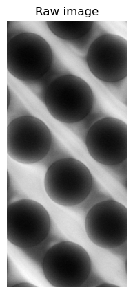
Then, we load the image file (in this case a TIFF-file), and display it.

import os
import numpy as np
import matplotlib.pyplot as plt
from skimage import exposure
import tifffile

#Set the path to the tif file
base_path = r'C:\Users\os4875st\Dropbox\PhD Tegenfeldt\.py\waves projects_shared\mp4_video_generation'
file_path = os.path.join(base_path,r'raw.tif')# Org path : E:\DNADLD_2022\T4_2022-06-15_2,3nguL\5mbar\100x_5mbar_out_013.nd2

#Read tif file

img = tifffile.imread(file_path)

#Show image
fig, ax = plt.subplots(figsize=(5,5))
ax.axis('off')
ax.imshow(img, cmap='gray') 
plt.title('Raw image')
plt.show()

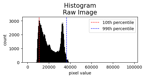
The contrast and brightness settings could be improved slightly. To get an overview of the pixel values in the image, see this pixel value histogram:

#Histogram
fontsize = 15
fig, ax = plt.subplots(figsize=(5,2))
I = img.ravel()
I = I[I != 0] 
plt.hist(I,bins=256, color='k', range=(0,1.5*2**16))
plt.title(f'Histogram\nRaw Image', fontsize=fontsize)
plt.xlabel('pixel value')
plt.ylabel('count')  
plt.show()

For exposure.rescale_intensity, we need to set the in_range and the out_range. The out_range will be uint-8 (unsigned 8 bit) as we don’t need larger images than that. The in_range we specify depending on what contrast we want. In the following example I set the in_range to be between the 10-th and 99-th percentile of array element values. See in the histogram where these percentiles correspond in the image.

#Select the percentile values to use for the limits
min = 10 #
max = 99 #99.9
min_val = np.percentile(img,min) #Returns the 10-th percentile of the array elements.
max_val = np.percentile(img,max) #Returns the 99-th percentile of the array elements.

#Show limits on the raw image histogram
fontsize = 15
fig, ax = plt.subplots(figsize=(5,2))
I = img.ravel()
I = I[I != 0] 
plt.hist(I,bins=256, color='k', range=(0,1.5*2**16))
plt.title(f'Histogram\nRaw Image', fontsize=fontsize)
plt.xlabel('pixel value')
plt.ylabel('count')  
plt.axvline(min_val, color='r', linestyle='dashed', linewidth=1, label=f'{min}th percentile')
plt.axvline(max_val, color='b', linestyle='dashed', linewidth=1, label=f'{max}th percentile')
plt.legend()
plt.show()

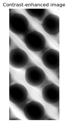
img_perc = exposure.rescale_intensity(img.copy(), in_range=(min_val, max_val), out_range='uint8')

#Show image
fig, ax = plt.subplots(figsize=(5,5))
ax.axis('off')
ax.imshow(img_perc, cmap='gray') 
plt.title('Contrast-enhanced image')
plt.show()

The image now has a slightly improved contrast:

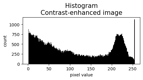
The histogram of this new image has then values between 0 and 255 as uint-8 images do:

# Histogram
fontsize = 15
fig, ax = plt.subplots(figsize=(5,2))
I = img_perc.ravel()
I = I[I != 0] 
plt.hist(I,bins=256, color='k', range=(0,255))
plt.title(f'Histogram\nContrast-enhanced image', fontsize=fontsize)
plt.xlabel('pixel value')
plt.ylabel('count')  
plt.show()

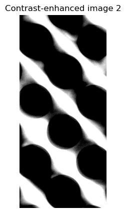
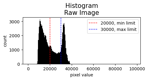
Another way to set the limits for exposure.rescale_intensity is to directly set the pixel values without bothering with percentiles. Percentiles are useful for a quick and dirty contrast enhancement. However, if minute differences in the percintiles lead to drastic image changes or the image is uneven in terms of bright and dark pixels, it makes sense to work directly with the pixel values. Below I select the in_range to between 20 000 and 30 000.

#Select the pixel values to use for the limits
min_val = 20000
max_val = 30000

#Show limits on the raw image histogram
fontsize = 15
fig, ax = plt.subplots(figsize=(5,2))
I = img.ravel()
I = I[I != 0] 
plt.hist(I,bins=256, color='k', range=(0,1.5*2**16))
plt.title(f'Histogram\nRaw Image', fontsize=fontsize)
plt.xlabel('pixel value')
plt.ylabel('count')  
plt.axvline(min_val, color='r', linestyle='dashed', linewidth=1, label=f'{min_val}, min limit')
plt.axvline(max_val, color='b', linestyle='dashed', linewidth=1, label=f'{max_val}, max limit')
plt.legend()
plt.show()

The resulting image has a much higher contrast, although perhaps too high of a contrast.

img_lims = exposure.rescale_intensity(img.copy(), in_range=(min_val, max_val), out_range='uint8')

#Show image
fig, ax = plt.subplots(figsize=(5,5))
ax.axis('off')
ax.imshow(img_lims, cmap='gray') 
plt.title('Contrast-enhanced image 2')
plt.show()